Energy Disaggregation.

Introduction

Energy disaggregation (also referred to as non-intrusive load monitoring or NILM) involves taking the aggregate energy signal from a household (for example, data from a smart meter), and inferring which devices/appliances are being used and how much they are using at any given point in time.

Background

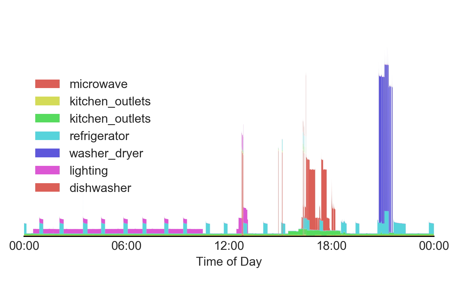
The Reference Energy Disaggregation Data Set (REDD) was released in 2011. It contains several weeks of power data for 6 different homes, along with data for individual appliance consumption for each house (typically around 15-20 devices).

In 2014, the Non Intrusive Load Monitoring Toolkit (NILMTK) was released. At the time, state of the art approaches relied on discrete methods, predominantly combinatorial optimization and factorial hidden Markov models.

In 2015, Jack Kelly released Neural NILM, applying neural networks to energy disaggregation, implementing autoencoders, LSTMs and a "rectangles" based approach (which I thought was a really novel and interesting one) on the UK DALE data set (another energy disaggregation data set). Broadly speaking, the autoencoders outperformed LSTMs. While the "rectangles" performance was comparable to autoencoders, it still enforced discreteness on the predictions and so we will ignore it for the purposes of our project.

Since Neural NILM, there have been a number of different deep learning efforts aiming to either improve on Jack Kelly's results, or implement his approaches on other data sets. In this project, I aim to improve on a traditional autoencoder approach by using variational autoencoders.

Why autoencoders don't really work

The general idea of an autoencoder is a neural network that takes some higher dimensional vector, encodes that vector to some lower dimensional space, decodes that encoded representation and tries to recover the same, original, high dimensional vector. In the energy disaggregation setting, instead of recovering the original energy signal, we try to recover an individual appliance signal.

While you usually see it as one network, there are really two parts here: an encoder and a decoder. People usually think about them in the context of compression and decompression, and this intuitively makes sense (i.e. reducing the dimensionality of your data).

The issue is in practice, they don't work particularly well for a lot of problems. The (very) general idea is that autoencoders tend to "cheat", memorizing vectors they are trained on by mapping them to a somewhat arbitrary point in the lower dimensional encoded space before decoding back to the original vector. While the weights will continue to adjust during training to minimize reconstruction error, the encoded representation itself isn't particularly meaningful. The consequences of this are:

1. Similar input vectors do not necessarily map to similar encoded vectors
2. Autoencoders are data-specific (i.e. they don't generalize well)

So how can we get more meaningful, generalizable latent representations of our input vectors, and will this also improve our reconstruction error?

Variational autoencoders

The simplest way to think about variational autoencoders is that we add Gaussian noise in the latent space to encourage efficient, meaningful representations of our data. With the addition of noise, our encoder is forced to map similar vectors to similar points in the latent space, so that our decoder can still get enough information from that latent representation to reconstruct a close approximation of those vectors.

We can't just add any old noise, however, otherwise our encoder could still map vectors arbitrarily far away so that the noise would have no bearing. In fact, we change the latent representation by encoding mean and standard deviation vectors and then sampling from it:

Furthermore, we add a penalty term to our loss function called the KL-divergence term. Without going into the derivation or math, this penalty term encourages our latent vector to approximate a unit Gaussian.

Now we can let the network decide the best trade-off between reconstruction error and ensuring that the latent representation is information-rich. The details of KL-divergence can be found elsewhere, but I couldn't find a visualization of the loss surface anywhere. So I made one quickly online below:

Above we can see that our KL-divergence term is at a minimum of 0 when the mean is 0 and standard deviation is 1 (i.e. the unit Gaussian). Furthermore, we see that our loss rapidly approaches infinity for small standard deviations.

Preliminary results

Long story short, variational autoencoders encourage more information-rich latent representations that generally outperform tradiational autoencoders. I've been able to use them for energy disaggregation, with improvements on REDD of around 20%:

In the coming weeks I'll be finishing the training on the top 5 appliances for each house to enable both better benchmark comparison, as well as some nicer visuals of disaggregated energy signals. Stay tuned!